Multi-version concurrency control
28 Jun 2020Multi-version histories
In conventional histories, at any point in time, there exists only one version of a data item. That means that the write operations always replace current version and the read operations always read the latest written version as it is defined by the schedule semantics:
\[w_1(x) w_2(x) r_3(x), H_s(r_3(x))\ =\ H_s(w_2(x))\]where \(H_s\) is a function that assigns every read the latest write to the corresponding data item.
Imagine that you can travel back in time. How it could look like?
\[w_1(x) r_3(x) w_2(x), H_s(r_3(x))\ =\ H_s(w_1(x))\]Here we send read \(r_3(x)\) back in time to read the output of the transaction \(t_1\).
How it could look like without commuting operations? The answer is simple: with the references to the previously written versions.
\[w_1(x_1) w_2(x_2) r_3(x_1), h(r_3(x)) = w_1(x)\]Here we have writes that create versions \(\{ x_1, x_2 \}\) of a data item \(x\). And the read that reads one version of \(t_1\). Function \(h\) is called a version function. With the version function the multi-version histories come into play.
Histories like one above are called multi-version (mv) histories. It is histories with defined version function that says who reads what. A read operation can read one of the previously written versions of a data item. If the version function always returns the latest version for reads the history called monoversion. Conventional histories are equivalent to corresponding monoversion variants.
This approach concludes multi-version concurrency control (MVCC) class of algorithms that are more powerful than conventional ones. They can produce more correct histories. Weikum & Vossen gives a great example of how much bigger the power of scheduling can be with the mv-histories. Consider the following history:
\[s = r_1(x) w_1(x) r_2(x) w_2(y) r_1(y) w_1(z) c_1 c_2\]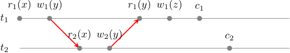
This history is not conflict-serializable due to the fact that \(r_1(y)\) arrived too late so it creates a cycle in the conflict graph of \(s\). This history could be serializable in example if \(r_1(y)\) came before \(w_2(y)\):
\[s_2 = r_1(x) w_1(x) r_2(x) r_1(y) w_2(y) w_1(z) c_1 c_2\]\(s_2\) does not have a cycle in the conflict graph so it is conflict-serializable. That’s cool. But we don’t control the order in which events arrive in our scheduler. What we control, is the point in time from which the read operation reads a version. We can define a version function so that serializability of \(s\) will become possible:
\[h(r_1(y)) = w_0(y)\]That means that \(r_1(y)\) will read the version of \(y\) written by the initial transaction \(t_0\) literally the previous version before \(t_2\):
\[m = r_1(x_0) w_1(x_1) r_2(x_1) w_2(y_2) r_1(y_0) w_1(z_1) c_1 c_2\]This multi-version history \(m\) is conflict equivalent to the:
\[m_2 = r_1(x_0) w_1(x_1) r_2(x_1) [ r_1(y_0) w_2(y_2) ] w_1(z_1) c_1 c_2\]in which we only commuted 2 operations. \(m_2\) is a monoversion history that is equivalent to \(s_2\) and \(s_2 \in CSR\):
\[s_2 = r_1(x) w_1(x) r_2(x) r_1(y) w_2(y) w_1(z) c_1 c_2\]Now when it is obvious that multi-versioning is a useful property let’s take a look at multi-version serializability.
Multi-version serializability
There are 2 kinds of MV serializability:
- MVSR - multi-version view serializability
- MCSR - multi-version conflict serializability
MVSR is defined by the analogy with the VSR: \(m \in MVSR\) if and only if there exists a serial monoversion schedule \(m'\) for the same set of transactions such that \(RF(m) = RF(m')\) where \(RF\) is a read-from relation.
The final state view in MVSR is not relevant anymore because any permutation of operations in \(s\) will produce the same final state view because writes do not erase previous versions.
MCSR by the analogy with CSR is a class in which for a history \(m\) there \(\exists\ m' - {serial\ monoversion}\) for the same set of transactions such that all conflict pairs of \(m\) occur in the same order in \(m'\).
An interesting nuance of the MV conflict set is its asymmetry: conflict set consists of the \((r_j(x_i), w_k(x_k))\) pairs such that \(w_i(x_i) <_m r_j(x_i) <_m w_k(x_k)\). So there are no ww and wr pairs in the mv-conflict set because commuting ww does not change anything for the following read operations, and commuting wr pairs does not affect the read variants space in a negative way so if the history with rw pair is serializable the one with the wr pair is serializable as well.
This asymmetry leads to the asymmetry in serializability class definition such that it’s \(m\) conflict pairs must occur in the same order in \(m'\), not the pairs from \(m'\). More details in [3]. I have spent some time reading out the definition of the MCSR in Vossen & Weikum book because they do not make an accent on that nuance from my point of view.
The relation between classes is as follows:
\(CSR \subset MCSR \subset MVSR \subset {histories} \\\) \(CSR \subset VSR \subset MVSR\\\)
On testing serializability
Let’s take a look at how a history may be tested for the multi-version serializability. We will start with testing for MCSR and then continue with the MVSR with this example:
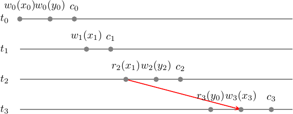
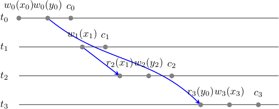
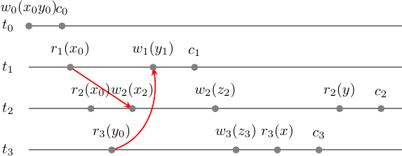
\[m = w_0(x_0) w_0(y_0) c_0 w_1(x_1) c_1 r_2(x_1) w_2(y_2) c_2 r_3(y_0) w_3(x_3) c_3\]Let’s draw a multi-version conflict graph (MVCG):
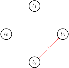
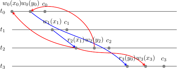
MVCG has no cycles and thus is acyclic. Hence \(m \in MCSR\). For even greater simplicity let’s take a look at the \(m\) step-graph along with the MV conflict set. It will show us in a graphical way where the single conflict edge \(x\) originates from and what we can commute to get serial monoversion history \(m'\) that will be \(m \approx_c m'\).
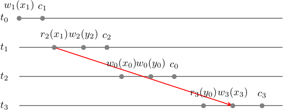
Now let’s commute something in \(m\) to find \(m'\) - serial monoversion history. What can confuse here is that the history \(m\) is already serial but not monoversion. Intuitively, what you would try to do first is to have \(m' = t_0 t_3 t_1 t_2\) but it is incorrect, because reverses conflict pair \((r_2(x_1), w_3(x_3))\) which we can’t commute. So the only chance we have is to move \(t_0\) forward, commuting operations 1-by-1:
\[m = w_0(x_0) w_0(y_0) c_0 w_1(x_1) c_1 r_2(x_1) w_2(y_2) c_2 r_3(y_0) w_3(x_3) c_3 \\ [ w_0(x_0) w_0(y_0) c_0 ] [ w_1(x_1) c_1 r_2(x_1) w_2(y_2) c_2 ] r_3(y_0) w_3(x_3) c_3 \\ [ w_1(x_1) c_1 r_2(x_1) w_2(y_2) c_2 ] [ w_0(x_0) w_0(y_0) c_0 ] r_3(y_0) w_3(x_3) c_3 \\ m' = w_1(x_1) c_1 r_2(x_1) w_2(y_2) c_2 w_0(x_0) w_0(y_0) c_0 r_3(y_0) w_3(x_3) c_3 \\ m' = t_1 t_2 t_0 t_3 \\ \approx \\ s' = w_1(x) c_1 r_2(x) w_2(y) c_2 w_0(x) w_0(y) c_0 r_3(y) w_3(x) c_3 \\ = t_1 t_2 t_0 t_3\]The fun part is that we moved our transactions \(t_1, t_2\) back in time behind the \(t_0\) that is an initial state transaction. However, commuting \(t_0\) did not prevent us from imagining the proper serial monoversion history even tho the whole thing is equivalent to the history in which we send scheduling transactions even further back in time.
The conflicts of \(m\) occur in the same order in \(m'\) so we are good:
We have proved that \(m \in MCSR\) and found serial monoversion \(m'\) such that \(m \approx_c m'\). Now let’s take a look at how \(m\) looks like in MVSR. We already know that \(MCSR \subset MVSR\) so \(m \in MCSR \Rightarrow m \in MVSR\).
But in any way, is it \(m'\) that we found for the MCSR case is sufficient for the MVSR. Let’s test it!
First of all, let’s prove that \(m \in MVSR\) on its own. We will build a multi-version serializability graph (MVSG) to see it is acycle. We can’t do that without defining a version order relation upfront. In any way, MVSR is defined as \(RF(m) = RF(m')\), so let’s start with the step-graph with read-from relation:
What you see here is 1/3 of the MVSG edges that consists of the conflict graph \(G(s)\) that are wr edges of the form \((w_i(x_i), r_j(x_i))\). The rest consists of the conflicts depending on the version order.
Now taking the version ordering from our \(m'\) MCSR case we are having:
\[x_1 << x_0 << x_3 \\ y_2 << y_0\]For \(r_2(x_1)\) we have \(w_1(x_1) <_{m'} r_2(x_1) <_{m'} w_0(x_0)\) and \(w_1(x_1) <_{m'} r_2(x_1) <_{m'} w_3(x_3)\) so we must add 2 edges to the MVSG: \(\{(r_2(x_1), w_0(x_0)), (r_2(x_1), w_3(x_3))\}\).
For \(r_3(y_0)\) we have \(w_2(y_2) <_{m'} w_0(y_0) <_{m'} r_3(y_0)\) so we must add an edge to the MVSG: \((w_2(y_2), w_0(y_0))\).
So we have got:
By collapsing operations into the transactions vertices we can obtain an MVSG:
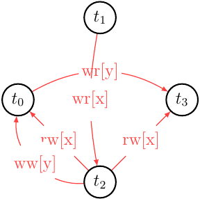
It’s easy to see it is acycle and that means \(m \in MVSR\) and the version order we picked based on \(m'\) serial monoversion history is good enough.
For more curiosity we can compare read-from sets of \(m, m'\):
\[m = w_0(x_0) w_0(y_0) c_0 w_1(x_1) c_1 r_2(x_1) w_2(y_2) c_2 r_3(y_0) w_3(x_3) c_3 \\ RF(m) = \{ (t_1, x, t_2), (t_0, y, t_3) \} \\ m' = w_1(x_1) c_1 r_2(x_1) w_2(y_2) c_2 w_0(x_0) w_0(y_0) c_0 r_3(y_0) w_3(x_3) c_3 \\ = t_1 t_2 t_0 t_3 \\ RF(m') = \{ (t_1, x, t_2), (t_0, y, t_3) \} \\ \Rightarrow \\ RF(m) = RF(m') \\ \Rightarrow \\ m \in MVSR\]And finally for those who are curious how the version function looks like for \(m\):
\[h(r_2(x)) = w_2(x) \\ h(r_3(y)) = w_0(y) \\ h(w_i(a)) = w_i(a)\]MVCC schedulers
We have seen what is MV serializability, how it is defined and works. Now it is time to take a look at algorithms that can produce mv-serializable schedulers. Let’s start with the following history sample:
\[s = r_1(x) r_2(x) r_3(y) w_2(x) w_1(y) c_1 w_2(z) w_3(z) r_3(x) c_3 r_2(y) c_2\]Let’s check if \(s\) is multi-version serializable and then we will see how the schedulers work. If \(s\) is mv-serializable it must have a version function that matches serializability criteria. But even before that, we can test it for mv-conflict/serializability graph acyclicity.
Here is our step-graph:
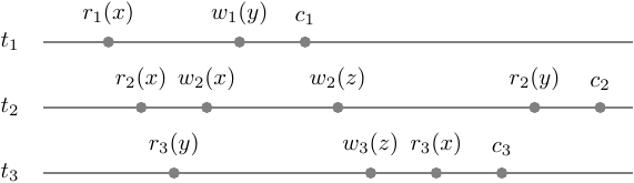
It is easy to imagine what possible mv-serializable schedule would likely have in conflicts and versions. The version function will map writes to unique variables versions anyway: \(h(w_i(a)) = w_i(a_i)\). Also, it will map reads to the latest versions at least if there are only single one of them: \(h(r_1(x)) = w_0(x_0)\), \(h(r_2(x)) = w_0(x_0)\), \(h(r_3(y)) = w_0(y_0)\).
We have drawn all possible mv-conflicts and even tho we did not define versions for \(\{ r_3(x), r_2(y) \}\) whatever they will be, they will not contribute to the mv-conflict set. Thus, we can pick any versions we like and let’s pick the latest committed.
\[m = w_0(x) w_0(y) c_0 r_1(x_0) r_2(x_0) r_3(y_0) w_2(x_2) w_1(y_1) c_1 w_2(z_2) w_3(z_3) r_3(x_1) c_3 r_2(y_1) c_2\]\(m\) mv-conflict graph is acycle and hence \(m \in MCSR \Rightarrow m \in MVSR\).
It’s easy to pick proper \(m'\) for \(m \in MCSR\) based on restrictions implied by the conflict edges:
\[t_1 < t_2, t_3 < t1 \\ \Rightarrow \\ t_3 < t_1 < t_2 \\ \Rightarrow \\ m' = t_0 t_3 t_1 t_2 \\ = w_0(x_0) w_0(y_0) c_0 [r_3(y_0) w_3(z_3) r_3(x_1) c_3] [r_1(x_0) w_1(y_1) c_1] r_2(x_0) w_2(x_2) w_2(z_2) r_2(y_1) c_2 \\ \approx \\ = w_0(x) w_0(y) c_0 [r_3(y) w_3(z) r_3(x) c_3] [r_1(x) w_1(y) c_1] r_2(x) w_2(x) w_2(z) r_2(y) c_2 \\ m' - {serial\ monoversion}\ | \\ r_1(x_0) <_m w_2(x_2) \land r_1(x_0) <_{m'} w_2(x_2) \\ r_2(y_0) <_m w_1(y_1) \land r_2(y_0) <_{m'} w_1(y_1) \\ \Rightarrow \\ MVCG(m) \subset MVCG(m') \\ \Rightarrow \\ m \in MCSR\]MVTO
Now, when we are sure that \(m\) is mv-serializable and what one possible variant of the version function looks like, let’s take a look at what we will get with the scheduling algorithms. We will start with the pessimistic non-locking MV Timestamp Ordering (MVTO) scheduler.
MVTO tracks a timestamp for every transaction that corresponds to its first operation.
For \(s\) we will have:
\[s = r_1(x) r_2(x) r_3(y) w_2(x) w_1(y) c_1 w_2(z) w_3(z) r_3(x) c_3 r_2(y) c_2 \\ r_1(x) <_s r_2(x) <_s r_3(y) \\ ts(t_1) < ts(t_2) < ts(t_3)\]Now we can produce an mv-schedule by outputting operations according to these rules:
- \[r_i(x) \to\ r_i(x_k)\ |\ w_k(x_k) < r_i(x) \land ts(t_k) < ts(t_i) \land i \neq k\]
- \[w_i(x) \to\ w_i(x_i)\ if\ \nexists\ step\ r_j(x_k)\ |\ ts(t_k) < ts(t_i) < ts(t_j), a_i\ otherwise\]
- \(c_i\) is delayed until all transactions that have written new versions of data items read by \(t_i\) have been processed.
Based on these rules we are getting:
| Input | Output | Rule |
|---|---|---|
| \(w_0(x)\) | \(w_0(x_0)\) | initial value |
| \(w_0(y)\) | \(w_0(y_0)\) | initial value |
| \(c_0\) | \(c_0\) | initial transaction |
| \(r_1(x)\) | \(r_1(x_0)\) | rule 1 |
| \(r_2(x)\) | \(r_2(x_0)\) | rule 1 |
| \(r_3(y)\) | \(r_3(y_0)\) | rule 1 |
| \(w_2(x)\) | \(w_2(x_2)\) | rule 2: \(\exists\ r_1(x_0)\ | ts(t_0) < ts(t_1) < ts(t_2)\) |
| \(w_1(y)\) | \(a_1\) | rule 2: \(\exists\ r_3(y_0)\ | ts(t_0) < ts(t_1) < ts(t_3)\) |
| \(w_2(z)\) | \(w_2(z_2)\) | rule 2: no one read z |
| \(w_3(z)\) | \(w_3(z_3)\) | rule 2: no one read z |
| \(r_3(x)\) | \(r_3(x_2)\) | rule 1 |
| \(c_3\) | wait \(t_2\) | rule 3: \(c_3\) delayed until \(t_2\) because \(r_3(x_2)\) was issued and \(t_2\) did not commit yet: \(t3 \to t2\) |
| \(r_2(y)\) | \(r_2(y_0)\) | rule 1 |
| \(c_2\) | \(c_2\) | rule 2: \(t_2\) did not read any uncommitted values |
| queued \(c_3\) | \(c_3\) | rule 3: \(t_2\) has been committed, so we can commit \(t_3\) |
Result is:
\[m = w_0(x_0) w_0(y_0) c_0 r_1(x_0) r_2(x_0) r_3(y_0) w_2(x_2) a_1 w_2(z_2) w_3(z_3) r_3(x_2) r_2(y_0) c_2 c_3 \\ \approx \\ m = w_0(x_0) w_0(y_0) c_0 r_2(x_0) r_3(y_0) w_2(x_2) w_2(z_2) w_3(z_3) r_3(x_2) r_2(y_0) c_2 c_3\]MVTO guarantees at least MVSR but we were lucky enough to get \(m \in MCSR\) with 1 transaction aborted:
\[m = w_0(x_0) w_0(y_0) c_0 r_2(x_0) r_3(y_0) w_2(x_2) w_2(z_2) w_3(z_3) r_3(x_2) r_2(y_0) c_2 c_3 \\ \approx_c \\ m' = t_0 t_2 t_3 \\\]MV2PL
MV2PL family of scheduling algorithms is based on conforming the 2PL rule: A transaction is said to satisfy the two-phase locking (2PL) protocol if all of its locking operations precede all of its unlock operations.
Most of them have different handling of the internal and the final steps of the transactions. Usually, they are relaxed on the write conflicts but the written versions must be certified.
In MV2PL transactions can write as many versions as they want but can read only the latest current version. Depending on the protocol variant the current version may allow reading only the latest certified committed versions or also an uncommitted version. The scheduler makes sure that at each point in time there is at most one uncommitted version of any data item.
MV2PL as well as 2V2PL uses 3 types of locks: read, write and certify. MV2PL uses the following locks compatibility matrix:
| Holder | \(r(x)\) | \(w(x)\) | \(c(x)\) | |
|---|---|---|---|---|
| Request | ||||
| \(r(x)\) | + | + | - | |
| \(w(x)\) | + | + | + | |
| \(c(x)\) | - | + | - |
That result into the following rules:
- If the step is not final within a transaction:
- (a) \(r_i(x) \to r_i(x_j)\) where \(x_j\) is the current version of the requested data item;
- (b) \(w_i(x) \to w_i(x_i)\) if there are no uncommitted versions of x, or waits otherwise
- If the step is final within transaction \(t_i\) it is delayed until the following
types of transactions are committed:
- (a) all those \(t_j\) that have read the data item written by \(t_i\)
- (b) all those \(t_j\) from which \(t_i\) has read
Applying these rules we are getting:
| Input | Output | Rule |
|---|---|---|
| \(w_0(x)\) | \(wl_0(x) w_0(x_0)\) | initial value |
| \(w_0(y)\) | \(wl_0(y) w_0(y_0)\) | initial value |
| \(c_0\) | \(cl_0(x) cl_0(y) ul_0 c_0\) | certify locks, full unlock, commit initial transaction |
| \(r_1(x)\) | \(rl_1(x) r_1(x_0)\) | rule (1.a) |
| \(r_2(x)\) | \(rl_2(x) r_2(x_0)\) | rule (1.a) |
| \(r_3(y)\) | \(rl_3(x) r_3(y_0)\) | rule (1.a) |
| \(w_2(x)\) | \(wl_2(x) w_2(x_2)\) | rule (1.b) |
| \(w_1(y)\) | \(wl_1(y) w_1(y_1)\) | rule (1.b) |
| \(c_1\) | wait \(t_3: rl_3(y)\) | rule (2.a): \(t_1\) must certify write \(w_1(y_1)\) before commit but \(y_0\) was read by \(t_3\) |
| \(w_2(z)\) | \(wl_2(z) w_2(z_2)\) | rule (1.b) |
| \(w_3(z)\) | \(wl_3(z) w_3(z_3)\) | rule (1.b) |
| \(r_3(x)\) | \(rl_3(x) r_3(x_0)\) | rule (1.a): let us not to allow dirty reads |
| \(c_3\) | \(cl_3(z) ul_3 c_3\) | rule (2) |
| \(r_2(y)\) | \(rl_2(y) r_2(y_0)\) | rule (1.a): let us not to allow dirty reads |
| \(c_2\) | wait \(t_1: rl_1(x)\) | rule (2.a): \(t_2\) must certify write \(w_2(x_2)\) before commit but \(x_0\) was read by \(t_1\) |
| deadlock \(\{ t_1, t_2 \}\) | we have a wait cycle: \(t_1 \to t_2 \to t_1\) |
Even though we know that \(s\) is mv-serializable MV2PL failed to produce a nice schedule for us. What we have got is only 1 committed transaction \(t_3\) and 2 deadlocked transactions.
2V2PL
2V2PL is an MV2PL variant in which the number of versions per item is limited by 2: pre-image and after-image. This is a nice property because it allows reducing storage utilization that is desirable for real-world implementations.
The algorithm also uses 3 locks but with different compatibility matrix [1] [4]:
| Holder | \(r(x)\) | \(w(x)\) | \(c(x)\) | |
|---|---|---|---|---|
| Request | ||||
| \(r(x)\) | + | + | - | |
| \(w(x)\) | + | - | - | |
| \(c(x)\) | - | - | - |
Derived rules are the same as in MV2PL. Scheduling for \(s\) will be the following:
| Input | Output | Rule |
|---|---|---|
| \(w_0(x)\) | \(wl_0(x) w_0(x_0)\) | initial value |
| \(w_0(y)\) | \(wl_0(y) w_0(y_0)\) | initial value |
| \(c_0\) | \(cl_0(x) cl_0(y) ul_0 c_0\) | certify locks, full unlock, commit initial transaction |
| \(r_1(x)\) | \(rl_1(x) r_1(x_0)\) | rule (1.a) |
| \(r_2(x)\) | \(rl_2(x) r_2(x_0)\) | rule (1.a) |
| \(r_3(y)\) | \(rl_3(x) r_3(y_0)\) | rule (1.a) |
| \(w_2(x)\) | \(wl_2(x) w_2(x_2)\) | rule (1.b) |
| \(w_1(y)\) | \(wl_1(y) w_1(y_1)\) | rule (1.b) |
| \(c_1\) | wait \(t_3: rl_3(y)\) | rule (2.a): \(t_1\) must certify write \(w_1(y_1)\) before commit but \(y_0\) was read by unfinished \(t_3\), so that \(t_3\) holds an incompatible read lock to the certify lock we want issue for \(t_1\) |
| \(w_2(z)\) | \(wl_2(z) w_2(z_2)\) | rule (1.b) |
| \(w_3(z)\) | wait \(t_2: wl_2(z)\) | rule (1.b): \(t_3\) must acquire write lock on \(z\), but there is incompatible lock held by \(t_2\) |
| \(r_3(x)\) | queued | blocked: \(t_3 \to t_2\) |
| \(c_3\) | queued | blocked |
| \(r_2(y)\) | \(rl_2(y) r_2(y_0)\) | rule (1.a) |
| \(c_2\) | wait \(t_1: r_1(x)\) | rule (2.a): \(t_2\) must certify write \(w_2(x_2)\) before commit but \(x_0\) was read by unfinished \(t_1\), so that \(t_1\) holds an incompatible read lock to the certify lock we want issue for \(t_2\) |
| all transactions deadlock | we have a wait cycle: \(t_1 \to t_3 \to t_2 \to t_1\) |
Even though we know that \(s\) is mv-serializable 2V2PL failed as well to produce a fine schedule. All transactions deadlocked in a loop involving all of them.
ROMV
ROMV goes even further than 2V2PL and offers a classical S2PL algorithm for update-transactions but optimizes read-only transactions with a non-blocking variant. It allows non-interfering long-running read-only transactions to be processed effectively - literally by reading versions committed before the start. It is especially useful for web applications that usually do more reads than writes.
It may be not applicable to all use cases because requires to classify transactions in advance into rw, ro categories.
The rules for the ROMV are as follows:
-
For update transactions: obey S/S2PL. It’s a classic 2PL plus the transactions must hold their write locks until the final step - commit. Versions timestamped by the time of the transaction commit.
-
For read-only transactions: Transactions acquire are timestamped by their beginning, unlike the update transactions. Read operations read the most recently committed versions right before their transaction timestamp.
S/S2PL is having the following compatibility matrix:
| Holder | \(r(x)\) | \(w(x)\) | |
|---|---|---|---|
| Request | |||
| \(r(x)\) | + | - | |
| \(w(x)\) | - | - |
So we are getting:
| Input | Output | Rule |
|---|---|---|
| \(w_0(x)\) | \(wl_0(x) w_0(x_0)\) | initial value |
| \(w_0(y)\) | \(wl_0(y) w_0(y_0)\) | initial value |
| \(c_0\) | \(ul_0 c_0\) | unlock, commit initial transaction |
| \(r_1(x)\) | \(rl_1(x) r_1(x_0)\) | |
| \(r_2(x)\) | \(rl_2(x) r_2(x_0)\) | |
| \(r_3(y)\) | \(rl_3(y) r_3(y_0)\) | |
| \(w_2(x)\) | wait \(t_1: rl_1(x)\) | \(wl_2(x)\) conflicts with \(rl_1(x)\) so \(t_2\) blocks for \(t_1\) |
| \(w_1(y)\) | wait \(t_3: rl_3(y)\) | \(wl_1(x)\) conflicts with \(rl_3(y)\) so \(t_1\) blocks for \(t_3\) |
| \(c_1\) | queued | blocked by \(t_3\) |
| \(w_2(z)\) | queued | blocked by \(t_1\) |
| \(w_3(z)\) | \(wl_3(z) w_3(z_3)\) | |
| \(r_3(x)\) | \(rl_3(x) r_3(x_0)\) | |
| \(c_3\) | \(ul_3 c_3\) | now \(t_1\) may proceed |
| \(w_1(y)\) q | \(wl_1(y) w_1(y_1)\) | |
| \(c_1\) q | \(ul_1 c_1\) | now \(t_2\) may proceed |
| \(w_2(x)\) q | \(wl_2(x) w_2(x_2)\) | |
| \(w_2(z)\) q | \(wl_2(z) w_2(z_2)\) | |
| \(r_2(y)\) | \(rl_2(y) r_2(y_0)\) | |
| \(c_2\) | \(ul_2 c_2\) |
Result is:
\[m = w_0(x_0) w_0(y_0) c_0 r_1(x_0) r_2(x_0) r_3(y_0) w_3(z_3) r_3(x_0) c_3 w_1(y_1) c_1 w_2(x_2) w_2(z_2) r_2(y_0) c_2\]ROMV guarantees at least MVSR but we were lucky enough to get \(m \in MCSR\) and all transactions committed:
\[m = w_0(x_0) w_0(y_0) c_0 [ r_1(x_0) r_2(x_0) ] r_3(y_0) w_3(z_3) r_3(x_0) c_3 w_1(y_1) c_1 w_2(x_2) w_2(z_2) r_2(y_0) c_2 \\ commute \\ = w_0(x_0) w_0(y_0) c_0 r_3(y_0) w_3(z_3) r_3(x_0) c_3 [ r_1(x_0) r_2(x_0) ] w_1(y_1) c_1 w_2(x_2) w_2(z_2) r_2(y_0) c_2 \\ commute \\ = w_0(x_0) w_0(y_0) c_0 r_3(y_0) w_3(z_3) r_3(x_0) c_3 r_1(x_0) w_1(y_1) c_1 [ r_2(x_0) ] w_2(x_2) w_2(z_2) r_2(y_0) c_2 \\ \Rightarrow m \approx_c m' = t_0 t_3 t_1 t_2\]MVSGT
I will leave it for homework.
MVSGT is similar to SGT and tracks the MV conflict graph in real-time to ensure serializability. MVSGT produces MCSR schedules.
Anomalies in SI
Snapshot isolation (SI) uses items versions to provide a consistent view (reads) of a database state (snapshot) at some point in time. Thus it requires MVCC. The thing is the resulting histories are not necessarily serializable.
For the details about what exactly SI is let’s turn to the work [6]:
-
A transaction \(t_i\) executing under SI conceptually reads data from the committed state of the database as of time \(start(t_i)\) (the snapshot). So it exploits reads as in ROMV for read-only transactions.
-
Snapshot Isolation must obey a “First Committer Wins” rule: the transaction may be committed only if there are no other transactions \(t_j\) that wrote data items that \(t_i\) wrote. It must be aborted otherwise.
Before [6] it was widely assumed that, under SI, read-only transactions always execute serializably provided the concurrent update transactions are serializable. They refuted it. Another possible anomaly is the Write Skew.
At this point, I would like to quote a definition of the SI by work [5]:
A system provides Snapshot Isolation if it prevents phenomena G0, G1a, G1b, G1c, PMP, OTV, and Lost Updates.
What we are left with are G2-item (write skew), G2 (write skew on predicates).
How the write skew looks like?
Write skew
\[m = w_0(x_0) w_0(y_0) c_0 r_1(x_0) r_2(x_0) r_1(y_0) r_2(y_0) w_1(x_1) c_1 w_2(y_2) c_2\]that can break \(f(x, y)\) invariant.
SSI
In 2012 it was shown how SI may be implemented to produce only serializable schedules. It’s called SSI [7].
References
- Transactional Information Systems: Theory, Algorithms, and the Practice of Concurrency Control and Recovery (The Morgan Kaufmann Series in Data Management Systems) 1st Edition.
- Managing Information Technology Resources in Organizations in the Next Millennium: 1999 Information Resources Management Association International Conference, Hershey, PA, USA, May 16-19, 1999.
- Algorithmic aspects of multiversion concurrency control by Thanasis Hadzilacos, Christos Harilaos Papadimitriou, march 1985.
- Information Systems Security: Third International Conference, ICISS 2007, Delhi, India, December 16-20, 2007, Proceedings.
- Scalable Atomic Visibility with RAMP Transactions, Peter Bailis, Alan Fekete, Ali Ghodsi, Joseph M. Hellerstein, and Ion Stoica, 2016.
- A Read-Only Transaction Anomaly Under Snapshot Isolation, By Alan Fekete, Elizabeth O’Neil, and Patrick O’Neil, 2004.
- Serializable Snapshot Isolation in PostgreSQL, Dan R. K. Ports, Kevin Grittner, 2012.